Simple Linear Regression

Learning Outcomes

Linear Regression
Ordinary Least Squares
R Code

R Packages

library(palmerpenguins)
library(tidyverse)

Linear Regression

Linear regression is used to model the association between a set of predictor variables (x’s) and an outcome variable (y). Linear regression will fit a line that best describes the data points.

Simple Linear Regression

Simple linear regression will model the association between one predictor variable and an outcome:

\[ Y = \beta_0 + \beta_1 X + \epsilon \]

\(\beta_0\): Intercept term
\(\beta_1\): Slope term
\(\epsilon\sim N(0,\sigma^2)\)

`palmerpenguins`

The palmerpenguins data set contains 344 observations of 7 penguin characteristics. We will be looking at different association of the penguins

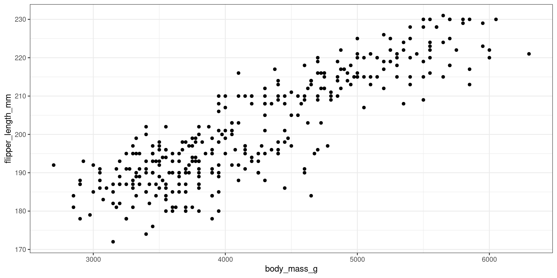
Scatter Plot

ggplot(penguins, aes(y = flipper_length_mm, x = body_mass_g)) +
  geom_point() + theme_bw()

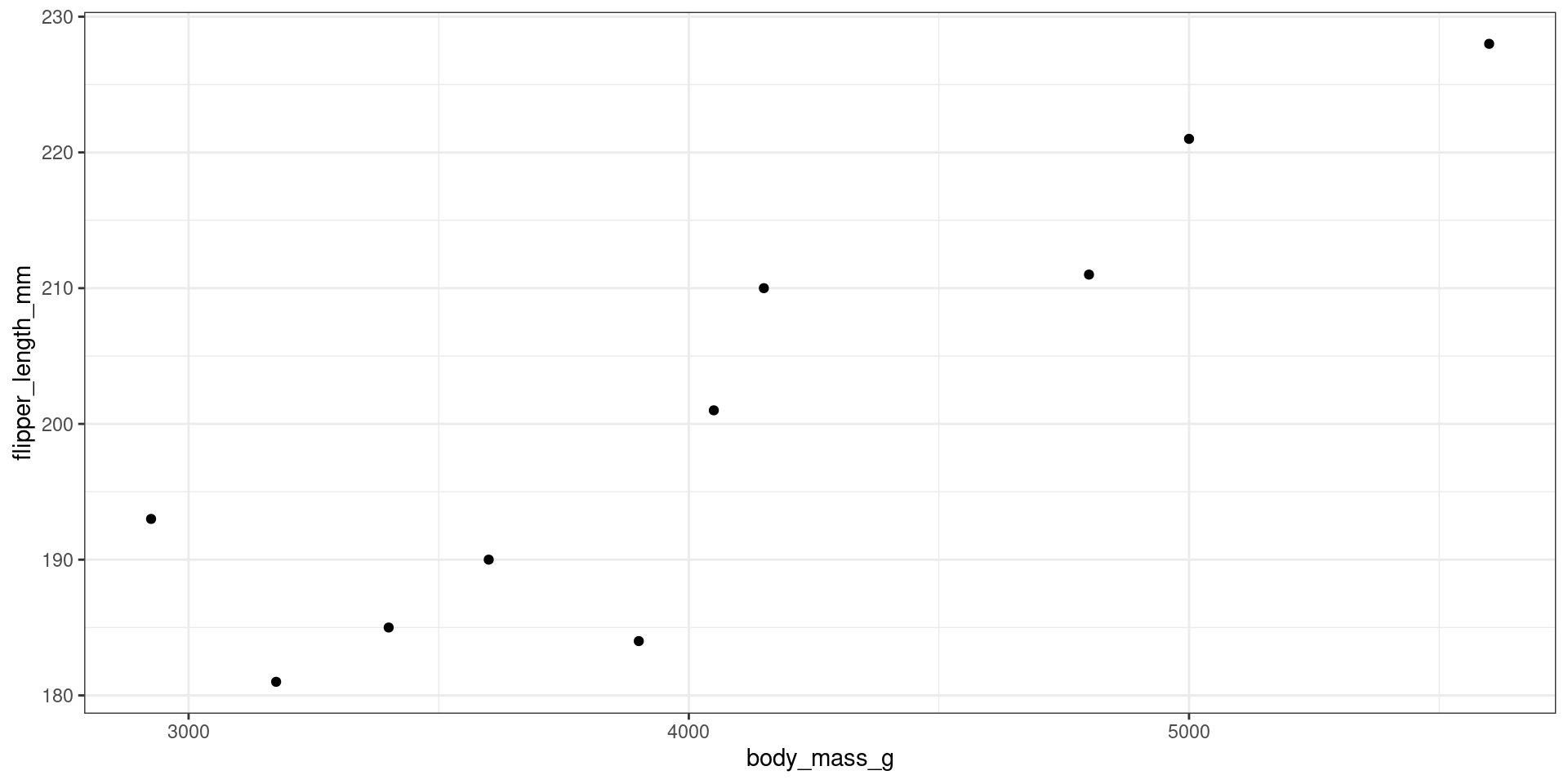
Scatter Plot

ggplot(sample_n(penguins,10), aes(y = flipper_length_mm, x = body_mass_g)) +
  geom_point() + theme_bw()

Fitting a Line

ggplot(penguins, aes(y = flipper_length_mm, x = body_mass_g)) + geom_point() + geom_smooth(method = "lm") +
  theme_bw() + annotate("text", label = "y=136.7+0.015x", x=3250, y=230, size = 10)

Interpretation

\[ \hat y = 136.73 + 0.015 x \]

Ordinary Least Squares

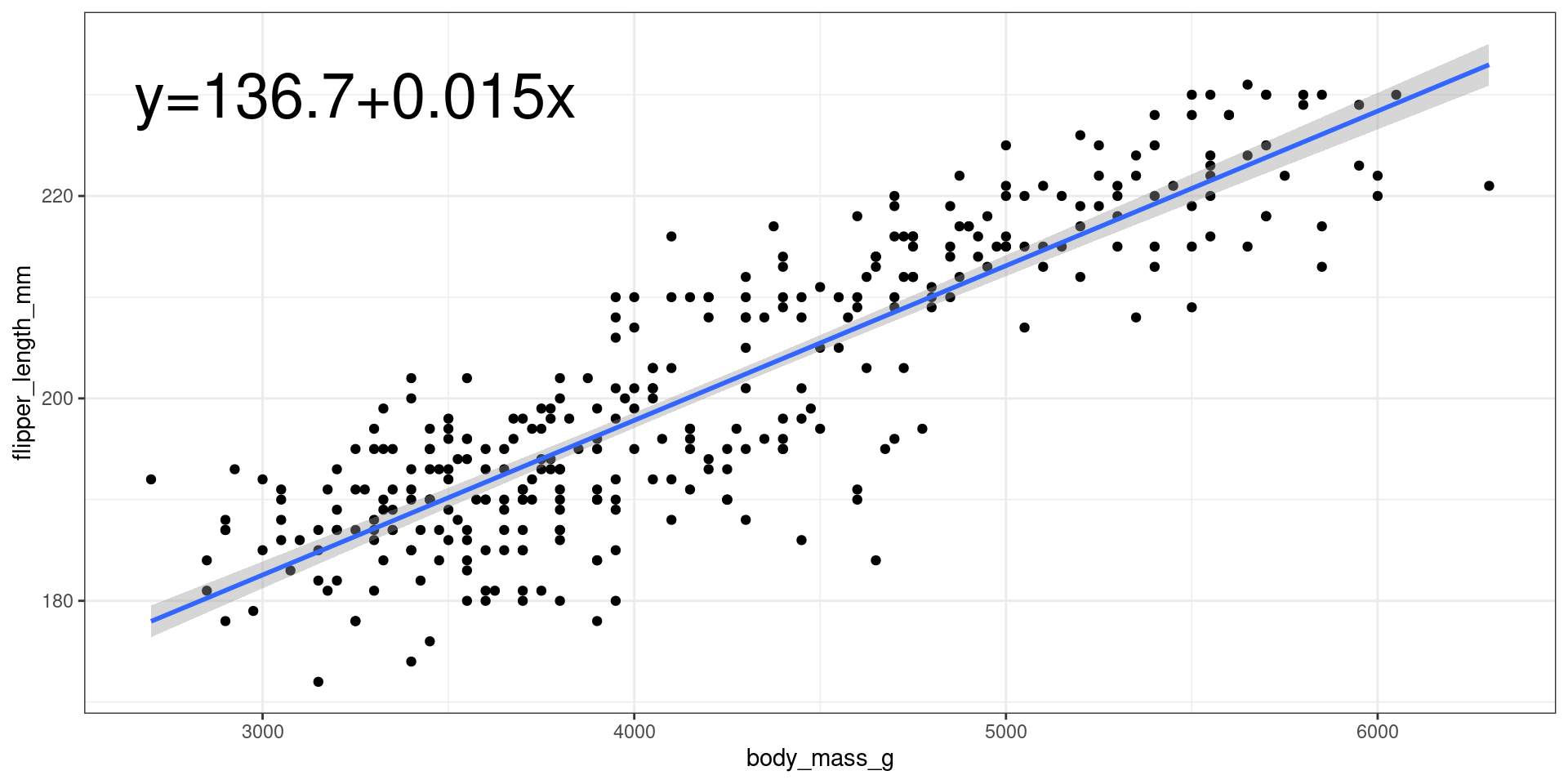
For a data pair \((X_i,Y_i)_{i=1}^n\), the ordinary least squares estimator will find the estimates of \(\hat\beta_0\) and \(\hat\beta_1\) that minimize the following function:

\[ \sum^n_{i=1}\{y_i-(\beta_0+\beta_1x_i)\}^2 \]

Estimates

\[ \hat\beta_0 = \bar y - \hat\beta_1\bar x \] \[ \hat\beta_1 = \frac{\sum^n_{i=1}(y_i-\bar y)(x_i-\bar x)}{\sum^n_{i=1}(x_i-\bar x)^2} \] \[ \hat\sigma^2 = \frac{1}{n-2}\sum^n_{i=1}(y_i-\hat y_i)^2 \]

Standard Errors of \(\beta\)’s

\[ SE(\hat\beta_0)=\sqrt{\frac{\sum^n_{i=1}x_i^2\hat\sigma^2}{n\sum^n_{i=1}(x_i-\bar x)^2}} \]

\[ SE(\hat\beta_1)=\sqrt\frac{\hat\sigma^2}{\sum^n_{i=1}(x_i-\bar x)^2} \]

Standard Error of \(\beta_0\)

File

Unbiasedness of \(\beta\)’s

Both \(\beta_0\) and \(\beta_1\) are unbiased estimators.

\(E(\beta_1)\)

Application in R

R Code

Use the lm() and summary() functions to fit a model and obtain the relevant statistics.

Fitting a line

p_lm <- lm(bill_depth_mm ~ bill_length_mm, data = penguins)
summary(p_lm)


Call:
lm(formula = bill_depth_mm ~ bill_length_mm, data = penguins)

Residuals:
    Min      1Q  Median      3Q     Max 
-4.1381 -1.4263  0.0164  1.3841  4.5255 

Coefficients:
               Estimate Std. Error t value Pr(>|t|)    
(Intercept)    20.88547    0.84388  24.749  < 2e-16 ***
bill_length_mm -0.08502    0.01907  -4.459 1.12e-05 ***
---
Signif. codes:  0 '***' 0.001 '**' 0.01 '*' 0.05 '.' 0.1 ' ' 1

Residual standard error: 1.922 on 340 degrees of freedom
  (2 observations deleted due to missingness)
Multiple R-squared:  0.05525,   Adjusted R-squared:  0.05247 
F-statistic: 19.88 on 1 and 340 DF,  p-value: 1.12e-05